Chapter 2.2: How to Diagnose Gearbox Noise Under Variable Speeds? — From STFT Spectrograms to Order Maps & Campbell Diagrams

In our previous chapter, Chapter 2.1: Why Does a Gearbox Ring Multiple Times in a Single Turn? — Shaft Frequencies, Mesh Harmonics, Sidebands & Order Tracking , we explored the four internal physical clocks of a constant-speed gearbox (shaft rotational frequency, gear mesh frequency, symmetric sidebands, and hunting tooth frequency) and introduced the foundational concept of angular resampling (order tracking).

However, the moment you step away from a constant-speed laboratory rig and onto a real factory floor or vehicle test bench, you immediately run into a major challenge: most precision actuators and gear reducers do not operate at a single, steady rotational speed:

1. Continuous Speed Sweeps (Run-up / Coast-down): Electric vehicle (EV) e-drive reducers, high-speed vacuum blowers, and drone gimbal motors accelerate continuously from $600\,\text{RPM}$ to $3000\,\text{RPM}$ (or tens of thousands of RPM). They may run whisper-quiet across most of the speed range, yet suddenly emit a piercing half-second “whine” or “howl” right as they pass through a specific speed (say, around $1950\,\text{RPM}$)—only for the noise to vanish immediately once past that speed;
2. Limited-Angle Reciprocating Strokes: Automotive HVAC damper actuators, power seat adjusters, flush door handles, LiDAR scanning mirrors, and smart-home pan-tilt heads are constrained by mechanical end-stops. They operate in repetitive cycles of “start-up acceleration $\rightarrow$ brief steady cruise $\rightarrow$ deceleration braking $\rightarrow$ dead-zone pause $\rightarrow$ reverse stroke.”

Under these variable-speed and non-stationary conditions, feeding a 10-second or 40-second microphone recording into a single standard FFT (Fast Fourier Transform)—just as you would for a constant-speed motor—is like taking a 10-second long-exposure photograph at the finish line of a 100-meter sprint. Every transient click, start-stop reversal thud, speed-drifting mesh tone, and fleeting housing resonance gets blended together into an unrecognizable blur.

To perform a “dynamic, high-definition CT scan” on variable-speed and reciprocating gearboxes, we must upgrade from a static 1D frequency spectrum to a 2D “moving picture” equipped with time and speed axes. Skipping heavy integral calculus, this chapter uses plain, intuitive shop-floor language to walk you through STFT Spectrograms (Waterfall Plots), Angle-Domain Order Maps, Campbell Diagrams, and Order Slices, showing you how ANSV Gear-NVH Intelligent Acoustic & Vibration Diagnostic System pinpoints hidden housing resonances and periodic impacts.

---

1. Why a Single Global FFT Goes Blind Under Variable Speeds: Three Fatal Blind Spots

A standard global FFT analyzer works in a very simple way: it takes your entire audio recording from start to finish and averages everything into a single summary chart. While it calculates steady-state frequencies with high precision, it completely throws away all “time” information—it can tell you that a certain frequency existed somewhere inside those 10 seconds, but it has no idea which second it occurred, what speed the motor was running at, or how long it lasted.

When applied to run-up/coast-down sweeps or reciprocating strokes, this “lump-sum” global FFT suffers from three fatal blind spots:

Variable-Speed / Non-Stationary Phenomenon	What Physically Happened?	How a Single Global FFT Distorts It	Shop-Floor Misdiagnosis Consequence
1. Frequency Drift During Speed Ramps	A 23-tooth gear accelerates from $600\,\text{RPM}$ to $3000\,\text{RPM}$, sweeping its mesh frequency from $230\,\text{Hz}$ to $1150\,\text{Hz}$	Spectral Smearing (Blurred & Flattened): The sharp mesh peak is smeared across a $920\,\text{Hz}$-wide band ($230 \sim 1150\,\text{Hz}$), dropping peak amplitude by $15 \sim 25\,\text{dB}$	Severe gear whine looks like a harmless, flat bump on the FFT, allowing defective units to slip past EOL inspection
2. Fleeting Resonance at a Critical Speed	A gear harmonic crosses a $1500\,\text{Hz}$ housing natural mode at $1957\,\text{RPM}$, howling loudly for just $0.3\,\text{s}$	Diluted by Quiet Intervals: The $0.3\,\text{s}$ burst is averaged across the full $12\,\text{s}$ recording (diluted $40\times$) and buried in background noise	Customers complain about acceleration howl, but engineers see no prominent peak on the global FFT
3. Asymmetric Forward/Reverse Strokes	Forward (CW) runs quietly, but Reverse (CCW) clicks due to abnormal worm axial end-play, separated by dead-zone pauses	Strokes & Dead Zones Mixed Together: End-stop braking impacts, dead-zone floor noise, and CW/CCW signals are all stacked on top of each other	Engineers cannot tell whether CW or CCW is noisy, or mistake normal end-stop bumps for broken gear teeth

How do we fix this “lump-sum averaging” problem? The solution is remarkably intuitive: instead of feeding the entire 12-second recording into one giant FFT, we use a narrow “sliding time window” to slice out a tiny chunk (say, $0.25$ seconds) at a time, compute a local FFT, slide the window forward step by step along the time axis, and stitch hundreds of local spectra side by side into a color map. This is the first core weapon of modern NVH diagnostics: the Short-Time Fourier Transform (STFT).

---

2. Short-Time Fourier Transform (STFT) & Time-Frequency Spectrograms (Waterfall Plots)

1. What Are Spectrograms and Waterfall Plots?

Once we slice an audio recording into hundreds of short time frames and compute the FFT for each frame, there are two common ways to visualize the result:

• Time-Frequency Spectrogram (2D Color Heatmap): The horizontal axis is Time (or Speed), the vertical axis is Frequency (Hz), and color brightness represents acoustic energy (for instance, in ANSV Gear-NVH 2027, deep purple indicates quiet background noise, emerald green indicates moderate energy, and bright yellow highlights intense peaks). Think of it as looking straight down from an airplane at a topographic contour map of a mountain range;
• 3D Waterfall Plot: Each time slice’s FFT curve is stacked diagonally one behind another, resembling a cascading waterfall.

Both plots contain the exact same underlying data. In day-to-day troubleshooting, however, the 2D top-down Spectrogram is often far more practical and precise than a 3D Waterfall Plot because taller peaks in the foreground never block peaks behind them, and you can align events directly against the time and RPM axes.

---

2. How Wide Should the Sliding Window Be? The Natural Seesaw Between Time and Frequency

When setting up an STFT spectrogram, the single most important parameter an engineer chooses is: how long should each sliding time window ($T_w$) be?

Here lies a fundamental rule of physics: frequency resolution ($\Delta f$, the finest frequency grid spacing) is strictly the inverse of the window time length ($T_w$):

$$\text{Frequency Grid Resolution } \Delta f = \frac{1}{\text{Window Length } T_w}$$

This creates an unavoidable seesaw between seeing “exact time” and seeing “exact frequency”:

• Window Too Short (e.g., $T_w = 0.04\,\text{s}$) — Crisp Time, Blurry Frequency: With a $40$-millisecond window, you can pinpoint the exact millisecond a “click” occurs. However, because the window is so brief, the frequency grid is a coarse $1 / 0.04 = 25\,\text{Hz}$! If a gear mesh peak has eccentricity sidebands spaced $20\,\text{Hz}$ apart (such as $22\text{X}$, $23\text{X}$, and $24\text{X}$), a $25\,\text{Hz}$ grid blurs them into one thick ribbon, making it impossible to see sideband modulation;
• Window Too Long (e.g., $T_w = 1.50\,\text{s}$) — Fine Static Frequency, Self-Smeared During Speed Ramps: Stretching the window to $1.5$ seconds refines the static frequency grid to $0.67\,\text{Hz}$. But during a speed ramp, the motor accelerates by $300\,\text{RPM}$ inside that single $1.5$-second window! Because the gear frequency at the end of the window is hundreds of Hertz higher than at the beginning, the diagonal order lines break apart into blurry, stair-stepped blocks.

To make this trade-off crystal clear, we used ANSV Gear-NVH to simulate a $23$-tooth gear accelerating linearly from $600\,\text{RPM}$ to $3000\,\text{RPM}$ over $12\,\text{s}$ (containing the $1\text{X}$ shaft frequency, $23\text{X}$ fundamental mesh tone with $22\text{X}/24\text{X}$ sidebands, $46\text{X}$ 2nd harmonic, $69\text{X}$ 3rd harmonic, and a $1500\,\text{Hz}$ housing natural mode). Compare how the exact same recording looks under three different window lengths:

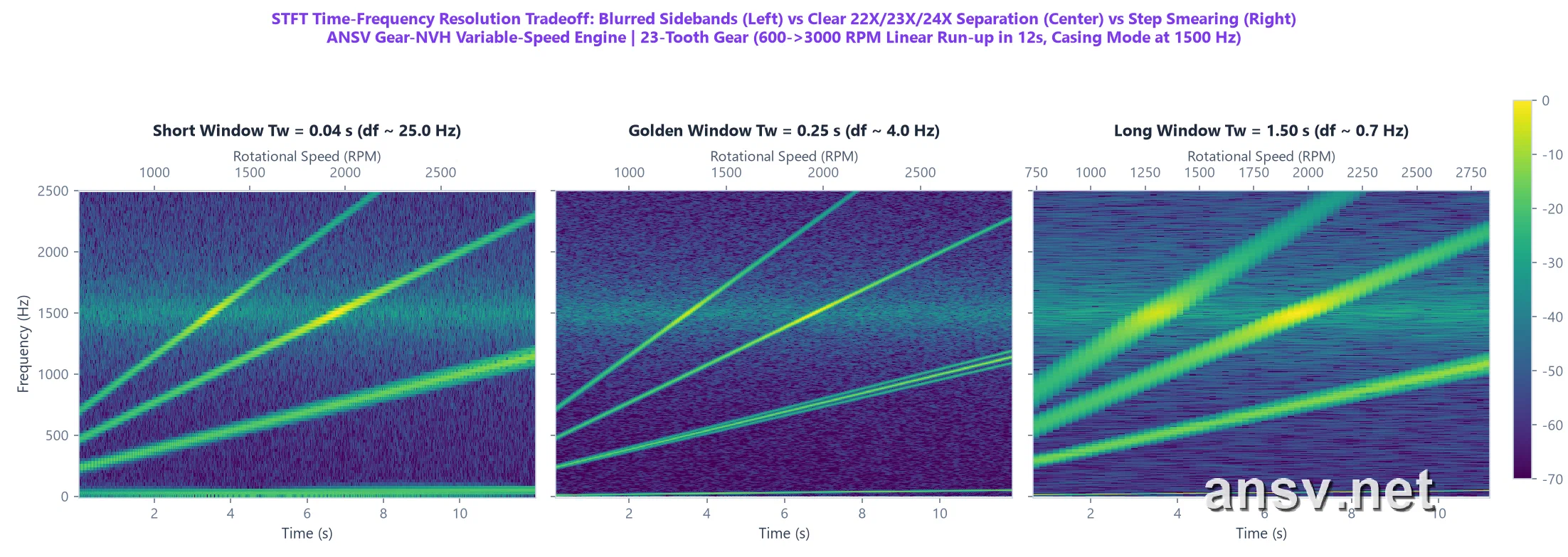▲ Figure 1: The exact same run-up audio analyzed under three STFT window lengths. Left ($T_w = 0.04\,\text{s}$): the frequency grid is too coarse ($25\,\text{Hz}$), merging $23\text{X}$ and its $22\text{X}/24\text{X}$ sidebands into a single thick band. Right ($T_w = 1.50\,\text{s}$): speed changes too much within each window, turning diagonal lines into blurry steps. Center (Golden Window $T_w = 0.25\,\text{s}$, $4\,\text{Hz}$ resolution): hits the sweet spot—tracking smooth diagonal speed ramps while cleanly separating the $23\text{X}$ carrier from its $22\text{X}$ and $24\text{X}$ sidebands!

💡TIP

Shop-Floor Rule of Thumb: Choosing Your STFT Window Length Keep this simple rule in mind: for normal slow run-up/coast-down sweeps ($150 \sim 300\,\text{RPM/s}$), setting the STFT window between $0.15 \sim 0.30\,\text{seconds}$ cleanly resolves 95% of gear whine harmonics and sidebands. Only shrink the window down to $0.02 \sim 0.05\,\text{seconds}$ when you specifically need to time-stamp millisecond-level hard tooth impacts. In ANSV Gear-NVH 2027, the engine automatically selects the optimal window for your operating speed range with zero manual tuning required.

---

3. Reading a Spectrogram at a Glance: Diagonal Lines, Horizontal Lines & Vertical Stripes

Once you have a clean STFT spectrogram, experienced NVH engineers don’t reach for complex math tables—they simply look at three line directions on the chart, because different mechanical faults leave completely different geometric footprints:

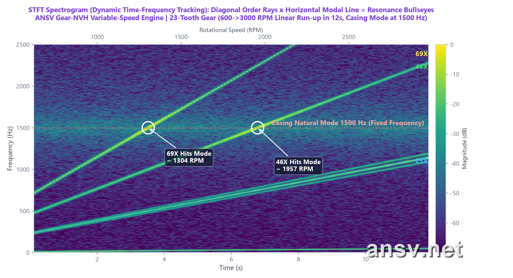▲ Figure 2: Decoding a run-up STFT spectrogram. The bright lines climbing diagonally from bottom-left to top-right ($23\text{X}$, $46\text{X}$, $69\text{X}$) are gear mesh tones that scale proportionally with shaft speed. The horizontal dashed red line sitting still at $1500\,\text{Hz}$ is the housing’s natural resonant frequency. Right where the $69\text{X}$ ray (at $1304\,\text{RPM}$) and $46\text{X}$ ray (at $1957\,\text{RPM}$) cross the $1500\,\text{Hz}$ horizontal line, the trace erupts into bright yellow—catching “gear order excitation hitting housing resonance” red-handed!

On any time-frequency spectrogram, remembering the “Diagonal, Horizontal, Vertical” rule lets you classify the root cause in under a minute:

Line Direction on Spectrogram	Why Does It Look Like This?	Physical Meaning	Common Mechanical Causes	Who Should Fix It? (Corrective Action)
1. Diagonal Lines (Climbing Up-Right)	As RPM rises, teeth mesh more times per second, so frequency climbs proportionally with speed	Rotating Order Excitation (Locked to Shaft Speed)	Gear mesh fundamental & harmonics ($23\text{X}, 46\text{X}$), eccentricity sidebands, rotor unbalance ($1\text{X}$)	Gear & Shaft Design: Apply tip relief / lead crowning, tighten gear radial runout, balance the rotor
2. Horizontal Lines (Flat & Stationary)	No matter how fast the motor spins, this frequency stays locked at a fixed Hertz like a tuning fork	Housing / Bracket Structural Resonance, or Power-Line Hum	Thin-wall plastic/aluminum casing natural mode, cantilevered bracket resonance, acoustic box standing wave, $50/60\,\text{Hz}$ electrical hum	Housing & Fixture Design: Never waste money re-cutting gear molds! Add stiffening ribs to thin casing walls, apply damping pads, or stiffen the test fixture
3. Vertical Stripes (Broadband Flashes)	A sharp, brief mechanical knock excites frequencies from near-zero up to tens of kHz all at the same instant	Periodic Hard Impact Pulses (“Clicking / Rattle”)	Single-tooth burr/ding/chipped tooth, excessive backlash reversal knock, bearing ball indentation, rotor axial end-play bump	Measure Time Spacing $\Delta t$ Between Stripes: e.g., a vertical stripe every $50\,\text{ms}$ means $20$ impacts/sec, directly indicting the shaft spinning at $20\,\text{rev/s}$ ($1200\,\text{RPM}$)!

---

3. From Angle-Domain Order Maps to Campbell Diagrams & Order Slices

Mastering the STFT spectrogram already puts you ahead of 80% of engineers who rely solely on static FFTs. Yet in multi-stage gearboxes or rapid speed sweeps, dozens of crisscrossing diagonal lines can still overwhelm the naked eye. To make the diagnosis of “diagonal order lines hitting horizontal modal lines” unmistakably clear, NVH engineers use a trio of tightly linked plots: the Order Map, the Campbell Diagram, and the Order Slice.

---

1. Angle-Domain Order Map: Straightening Every Diagonal Line into a Horizontal Line

Why do gear tones appear as diagonal lines in Figure 2? Because our vertical axis measures events per second ($\text{Hz}$); as the shaft speeds up, more teeth pass per second, so the line slopes upward. What if we change how we count—instead of plotting “vibrations per second ($\text{Hz}$)” on the vertical axis, we plot “vibrations per shaft revolution (Order / $\text{X}$)”? This technique is called Computed Order Tracking (COT / Angular Resampling), where the signal is sampled at fixed shaft rotation angles rather than fixed time intervals.

The moment we switch the vertical axis to Order ($\text{X}$), something remarkable happens:

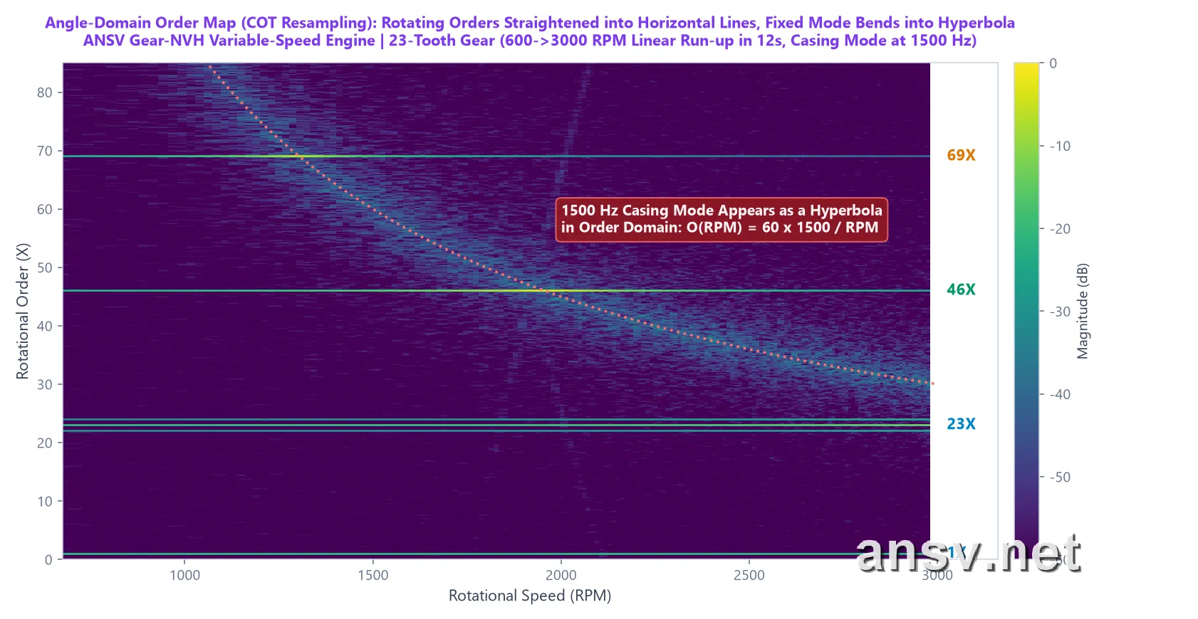▲ Figure 3: The Angle-Domain Order Map after angular resampling. Because a 23-tooth gear always meshes exactly 23 times per shaft turn—whether at $600\,\text{RPM}$ or $3000\,\text{RPM}$—every sound tied to the gears and shafts ($1\text{X}$, $22\text{X}$, $23\text{X}$, $24\text{X}$, $46\text{X}$, $69\text{X}$) is straightened into a perfectly flat horizontal line, completely immune to speed smearing! Conversely, the fixed $1500\,\text{Hz}$ housing mode bends into a curved red dashed line (a hyperbola).

The diagnostic rule on an Order Map could not be simpler: anything running dead-flat horizontally is 100% generated by rotating gears and shafts; anything curving downward is 100% a fixed-frequency structural resonance or external electrical interference!

---

2. The Campbell Diagram: Pinpointing Exact Resonance Speeds in One Second

A century ago, General Electric (GE) engineer Wilfred Campbell invented the famous Campbell Diagram to figure out why steam turbine blades were snapping at specific operating speeds. Today, it remains the ultimate compass for catching structural resonances in automotive transmissions, EV e-drives, and precision actuators.

Reading a Campbell Diagram is straightforward (horizontal axis = Speed in RPM, vertical axis = Frequency in Hz):

1. Diagonal Rays Fanning Out from the Bottom-Left: Represent the gear orders (such as $23\text{X}$ fundamental, $46\text{X}$ 2nd harmonic, $69\text{X}$ 3rd harmonic), whose frequencies climb proportionally with RPM;
2. Horizontal Red Line: Represents the housing’s natural resonant frequency (e.g., $1500\,\text{Hz}$ in this example, fixed like a tuning fork);
3. Colored Circles Along the Rays: The larger and brighter yellow the circle, the louder the sound at that exact speed and frequency.

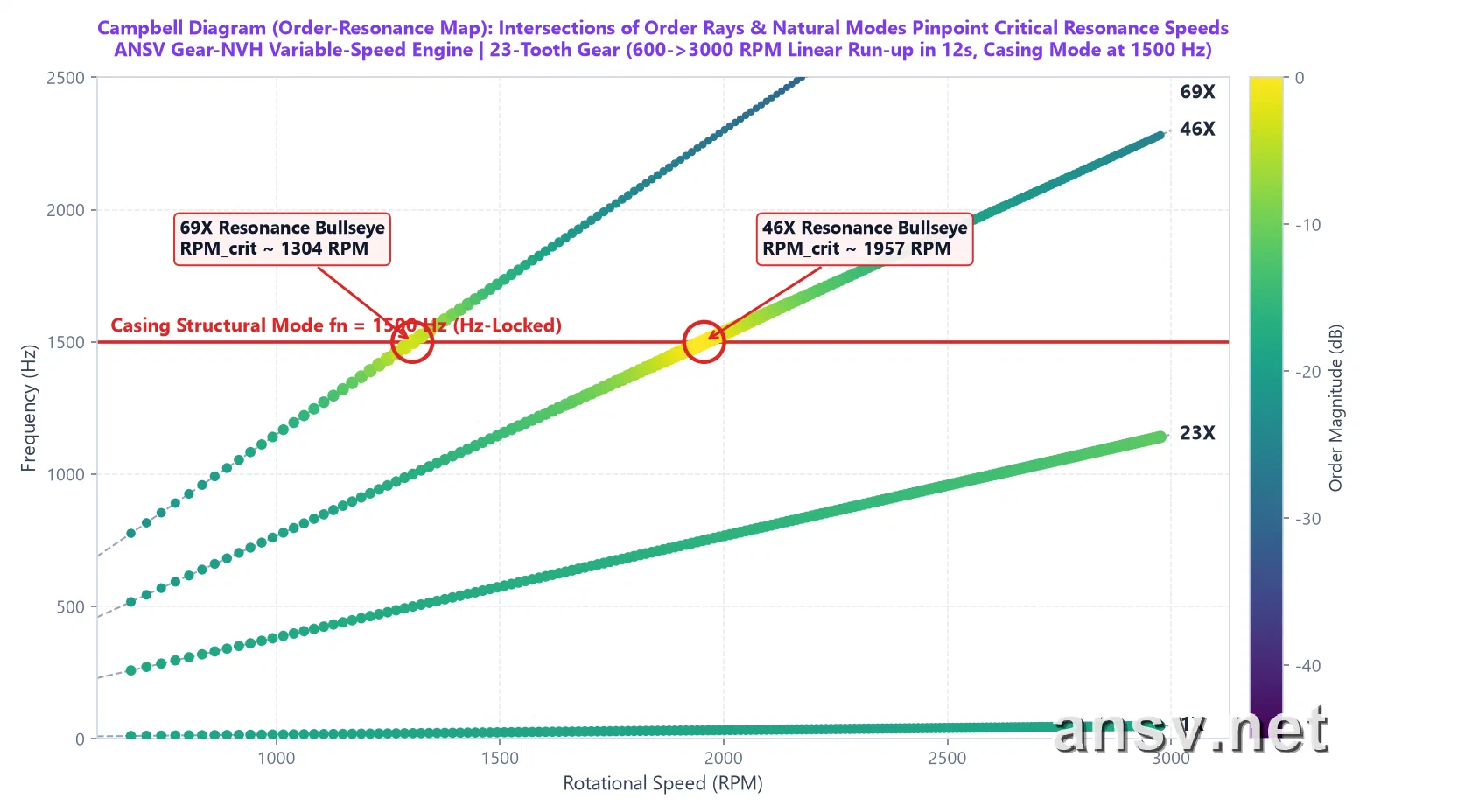▲ Figure 4: Campbell Diagram of the 23-tooth gear run-up. Follow the circles along the $69\text{X}$ and $46\text{X}$ diagonal rays: across most speeds, the circles are small and dark green. However, right at the two red-circled intersections where those rays cross the $1500\,\text{Hz}$ housing mode ($1304\,\text{RPM}$ and $1957\,\text{RPM}$), the circles balloon into bright yellow bullseyes!

How do you calculate those exact critical resonance speeds? All it takes is simple elementary-school division:

$$\text{Critical Resonance Speed (RPM)} = \frac{60 \times \text{Casing Natural Frequency (Hz)}}{\text{Gear Order (X)}}$$

Let’s do the mental math for our 23-tooth gear and $1500\,\text{Hz}$ housing mode in Figure 4:

• 3rd Harmonic ($69\text{X}$) hitting $1500\,\text{Hz}$: $60 \times 1500 \div 69 = \mathbf{1304\,\text{RPM}}$;
• 2nd Harmonic ($46\text{X}$) hitting $1500\,\text{Hz}$: $60 \times 1500 \div 46 = \mathbf{1957\,\text{RPM}}$;
• Fundamental ($23\text{X}$) hitting $1500\,\text{Hz}$: $60 \times 1500 \div 23 = \mathbf{3913\,\text{RPM}}$ (well above the $3000\,\text{RPM}$ maximum operating speed, so the fundamental never triggers resonance within the operating range!).

This completely solves the mystery from the beginning of the chapter: why is this gearbox whisper-quiet at $1000\,\text{RPM}$ and $2500\,\text{RPM}$, yet screams briefly when passing $1304\,\text{RPM}$ and $1957\,\text{RPM}$? Because at those two exact speeds, the gear’s higher harmonics land squarely on the housing’s “tuning-fork frequency”! Re-cutting the gear mold here would be a complete waste of money; the right engineering fix is to add a stiffening rib to the housing wall to push its natural frequency out of the operating speed range.

---

3. Order Slices: Pulling Out Each Order’s Volume Curve Against RPM

To compare the exact decibel level of each harmonic across the speed range, we can trace along the $23\text{X}$, $46\text{X}$, and $69\text{X}$ rays in Figure 4 and plot their amplitudes as three clean “Amplitude (dB) vs. Speed (RPM)” curves, known as Order Slices:

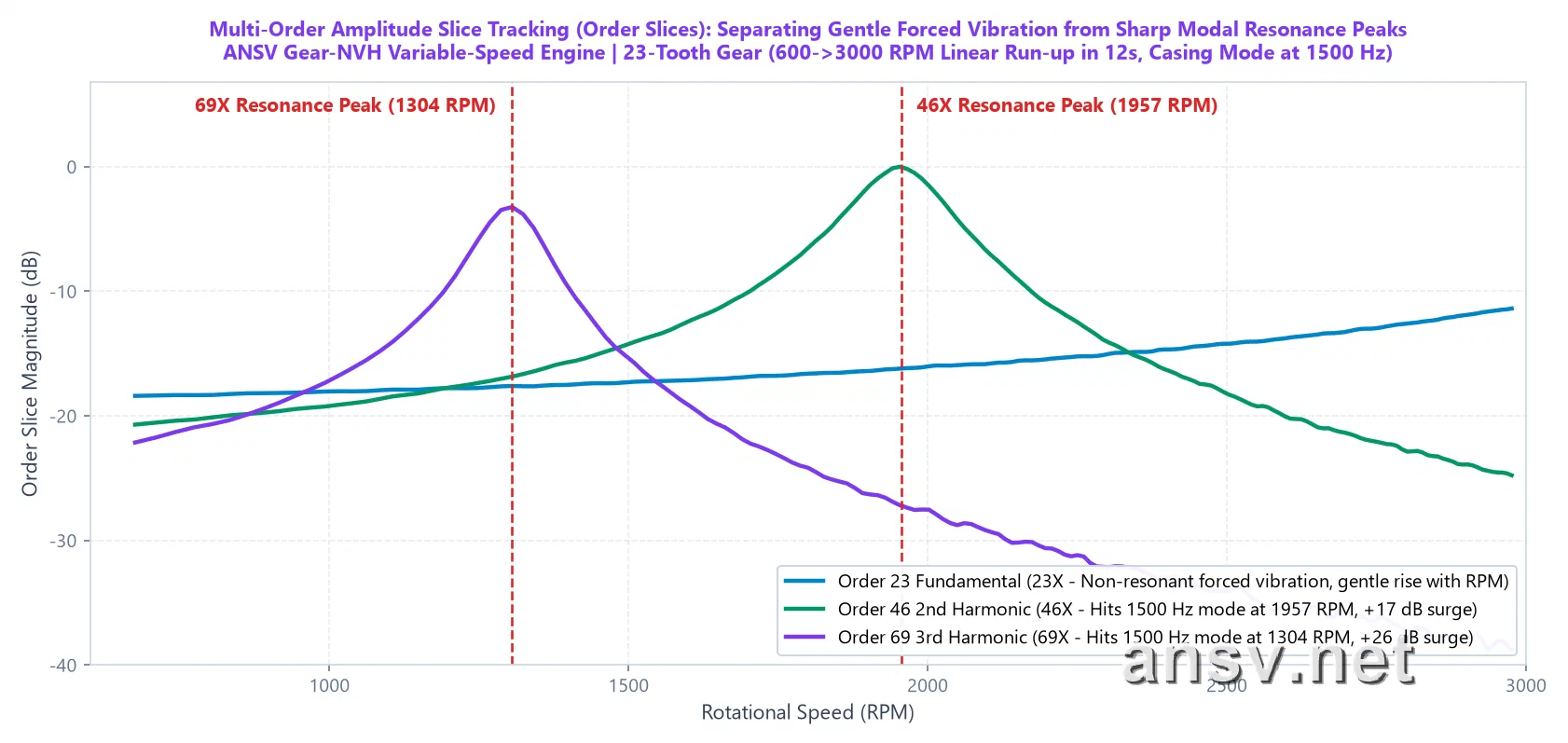▲ Figure 5: Order Slice curves tracking the amplitude of $23\text{X}$ (blue), $46\text{X}$ (green), and $69\text{X}$ (purple) across the entire speed sweep.

Looking at the three curves in Figure 5, anyone can immediately tell the difference between “normal speed-dependent growth” and “structural resonance amplification”:

1. Blue Curve ($23\text{X}$ Mesh Fundamental) — Normal Forced Mechanical Vibration: Because $23\text{X}$ never touches the $1500\,\text{Hz}$ housing mode below $3000\,\text{RPM}$, its curve shows no sharp spikes—just a smooth, gentle rise of about $7\,\text{dB}$ as rotational kinetic energy increases;
2. Green Curve ($46\text{X}$) & Purple Curve ($69\text{X}$) — Caught-in-the-Act Housing Resonance Peaks: In non-resonant speed zones (such as $800\,\text{RPM}$ or $2800\,\text{RPM}$), the 2nd and 3rd harmonics are much quieter than the fundamental (blue line). Yet right at $1304\,\text{RPM}$ and $1957\,\text{RPM}$, housing resonance acts like a megaphone—amplifying these otherwise weak harmonics by $17 \sim 26\,\text{dB}$ ($7\times$ to $20\times$ higher sound pressure amplitude) so they tower over the fundamental!

---

4. Practical Implementation: How to Catch Resonance with a Slow Speed Sweep—Without a Tachometer

At this point, many engineers ask a very practical question: “The theory makes total sense, but traditional Order Maps and Campbell Diagrams require sticking reflective tape on the motor shaft and setting up an expensive laser tachometer (Keyphasor). Our micro-gearboxes and automotive actuators are fully enclosed—there’s nowhere to measure shaft pulses. How can we generate these plots?”

Moreover, many production test operators are used to fixing a DC power supply at a single voltage (say, a constant $1200\,\text{RPM}$) to record audio. Yet a constant-speed recording only plots a single vertical column of dots on a Campbell Diagram—it cannot trace diagonal order rays across speeds, and it completely misses housing resonances hiding at $1426\,\text{RPM}$ or $1565\,\text{RPM}$!

To solve both pain points on the shop floor, we use a streamlined “Slow Run-up/Coast-down Sweep + Tacholess Audio Ridge Tracking” workflow:

1. Slow Run-up / Coast-down Sweep: Adjust a programmable power supply (or PWM ramp) so the gearbox accelerates smoothly from low speed (e.g., $600\,\text{RPM}$) to high speed (e.g., $1800 \sim 2400\,\text{RPM}$) over $5 \sim 10\,\text{seconds}$, then coasts down slowly. This uses the gear teeth themselves as a continuous swept-sine shaker, tapping every structural mode of the housing from low to high frequency;
2. Tacholess Instantaneous RPM Extraction from Pure Audio: Inside ANSV Gear-NVH 2027’s standalone [⚡ Tacholess Order Tracking & Campbell Modal Resonance Workbench], no optical encoder is needed! Using a Viterbi optimal path-tracking algorithm, the software locks onto the gear mesh harmonics directly from the microphone recording, reconstructs the millisecond-by-millisecond instantaneous speed curve $\text{RPM}(t)$, performs angular resampling internally, and generates the complete 4-panel diagnostic suite in one click:

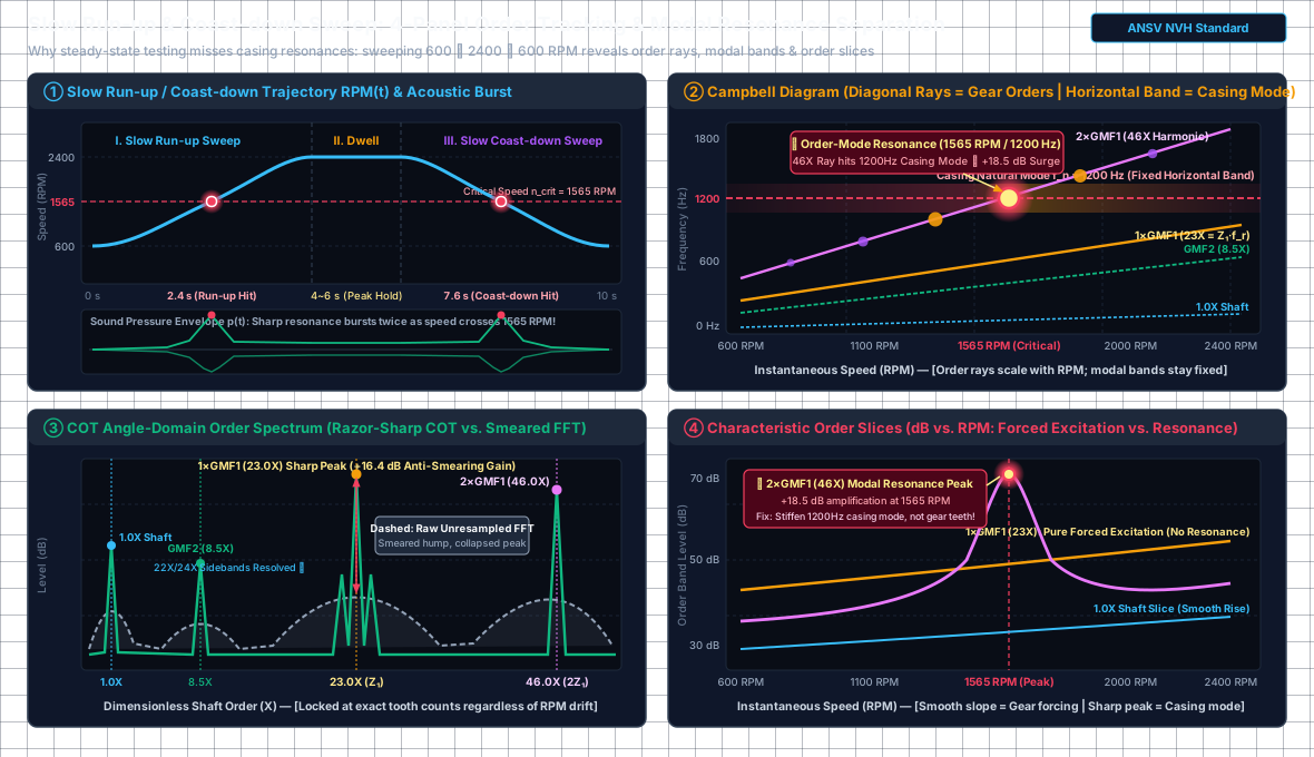▲ Figure 6: Slow Run-up / Coast-down Sweep ($600 \rightarrow 2400 \rightarrow 600\,\text{RPM}$) 4-panel diagnostic schematic: Top-Left (①) shows symmetrical acoustic resonance bursts at $2.4\,\text{s}$ (run-up) and $7.6\,\text{s}$ (coast-down) whenever the speed crosses $1565\,\text{RPM}$; Top-Right (②) Campbell diagram pinpoints the bullseye where the $46\text{X}$ order ray crosses the $1200\,\text{Hz}$ housing mode; Bottom-Left (③) COT angular resampling collapses the smeared traditional FFT hump (dashed gray) into a razor-sharp order peak (solid green, $+16.4\,\text{dB}$ gain); Bottom-Right (④) Order slices quantify the $+18.5\,\text{dB}$ resonance spike of $46\text{X}$ at $1565\,\text{RPM}$.

Below is the actual workbench screen after dragging a real $795 \rightarrow 1846\,\text{RPM}$ slow run-up recording into ANSV Gear-NVH 2027:

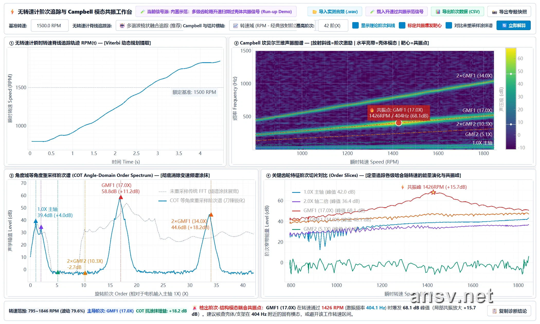▲ Figure 7: ANSV Gear-NVH 2027 standalone [⚡ Tacholess Order Tracking & Campbell Modal Resonance Workbench] live output: Top-Left (①) automatically extracts the $795 \rightarrow 1846\,\text{RPM}$ run-up speed profile from pure audio; Top-Right (②) Campbell diagram locks onto the Stage 1 mesh $\text{GMF}_1$ ($17.0\text{X}$) housing resonance bullseye at $1426\,\text{RPM}$ ($404\,\text{Hz}$, peak $68.1\,\text{dB}$); Bottom-Left (③) COT order spectrum sharpens the smeared FFT peak by $+18.2\,\text{dB}$; Bottom-Right (④) Order slice highlights the $+15.7\,\text{dB}$ resonance surge at $1426\,\text{RPM}$ and outputs automated engineering recommendations at the bottom!

---

4. Industrial Case Study & Software Workbench: 4-Stage Compound Gear Actuator (Total Ratio 495.4) End-to-End Troubleshooting

In real-world production lines and customer quality arbitration, beyond continuous run-up resonance sweeps (Campbell analysis), engineers frequently encounter limited-angle reciprocating actuators (multi-stroke segmentation), low-frequency periodic hard knocks hidden underneath high-frequency structural ringing (STFT vertical stripes + Hilbert envelope pulse stopwatch), and supplier responsibility disputes (“Is the noise coming from the drive motor itself or from gear meshing?”).

To keep this chapter focused, we have compiled the complete 8D root-cause investigation of a 4-stage compound gear actuator (two worm stages + two spur gear stages, total ratio $495.4$)—covering reciprocating 4-stroke segmentation, STFT & Hilbert envelope tracking of a $\Delta t = 50.1\,\text{ms}$ ($20.0\,\text{Hz}$) periodic impact, 5-speed verification ($360 \rightarrow 1900\,\text{RPM}$), bare-motor no-load decoupling (saving tens of thousands of dollars in unnecessary gear mold modifications in 20 minutes), and the ANSV Gear-NVH 2027 Intelligent Diagnostic Workstation 7-day free trial—into our dedicated feature article below:

👉 Read the Full Industrial Case Study & Software Feature Guide:
Gear-Acoustic: Mechanical Noise & Multi-Stage Transmission FFT Spectral Intelligent Diagnostic System (Full 4-Stage Gearbox Case Study & Free Trial)

---

5. Chapter Summary: The 3-Step Visual Playbook for Variable-Speed & Reciprocating NVH

Reviewing this chapter, whenever you face abnormal gearbox noise under variable speeds (run-up/coast-down sweeps) or non-stationary motion (reciprocating strokes), you don’t need to memorize complex calculus. Simply follow this 3-step visual playbook at the test bench to see straight through to the physical root cause:

1. Ditch the Single Global FFT—Look for “Diagonal, Horizontal, Vertical” on the STFT Spectrogram:
   • Under changing speeds or reciprocating strokes, a single long-window FFT smears drifting frequencies into flat bumps and dilutes brief resonances;
   • Switch to a time-resolved STFT Spectrogram (using a $0.15 \sim 0.30\,\text{s}$ golden window for slow speed ramps) and classify the three line directions:
     • Diagonal lines climbing up-right = Gear mesh & shaft orders locked to rotational speed (fix the gears and shafts);
     • Horizontal lines sitting flat = Housing / bracket natural modes locked to a fixed frequency (stiffen or damp the housing—never blindly re-cut gear molds!);
     • Vertical broadband stripes = Crisp, periodic hard impact pulses (measure the time interval $\Delta t$ between stripes to identify exactly which shaft is knocking once per revolution).
2. Straighten Diagonal Lines on the Order Map & Pinpoint Resonance RPM on the Campbell Diagram:
   • Through angular resampling (sampling at fixed rotation angles), all gear- and shaft-locked tones straighten into flat horizontal lines on the Order Map, eliminating speed smearing;
   • On the Campbell Diagram, the intersection where a diagonal gear order ray crosses a horizontal housing modal line marks the critical resonance speed (mental math formula: $\text{Resonance RPM} = 60 \times \text{Modal Frequency Hz} \div \text{Gear Order X}$);
   • Pair this with Order Slices to inspect individual order amplitudes: a gentle upward slope indicates normal forced vibration, whereas a sharp $15 \sim 25\,\text{dB}$ mountain peak at a specific RPM is unmistakable structural resonance.
3. Upgrade Your Test Method: Replace Single-Speed Spot Checks with a 5–10s Slow Speed Sweep:
   • During R&D validation or customer return investigations, don’t just record audio at one fixed nominal voltage (which only gives you a single isolated dot on a Campbell diagram);
   • Make it a habit to run a 5-to-10-second slow run-up / coast-down sweep. Paired with ANSV Gear-NVH ’s tacholess ridge-tracking workbench, you can map out every gear order whine and housing resonance across the entire operating speed range in one sweep—without sticking reflective tape or mounting an optical encoder!

---

📚 Further Reading & Handbook Navigation

• 🔙 Previous Chapter: 2.1 Why Does a Gearbox Ring Multiple Times in a Single Turn? — Shaft Frequencies, Mesh Harmonics, Sidebands & Order Tracking
• 🏠 Handbook Index: Gearbox NVH & Mechanical Noise Diagnostic Handbook
• 💻 Software Case Study & Free Trial: Gear-Acoustic: Industrial Multi-Stage Transmission FFT Spectral Intelligent Diagnostic System

Citation and Technical Discussion Notice

Author: Tony Chen | Digital R&D Expert in Micro Electromagnetic Actuators

Original source: ansv.net

Article URL: https://ansv.net/en/knowledge-base/gear-acoustic-nvh/07-stft-waterfall-order-spectrum-and-campbell-diagram/

Copyright: Unless otherwise stated, this article's original text, formulas, and original illustrations are licensed under CC BY-NC-ND 4.0 (Attribution—NonCommercial—NoDerivatives). Non-commercial sharing is welcome with attribution and a link to the original; adaptation, alteration, or excerpting is not permitted.

Unless expressly stated otherwise, third-party trademarks, patent figures, product images, and other third-party materials are not covered by this CC license. Their rights remain with their respective owners.

For technical inquiries or discussion, feel free to contact [email protected].